Department of Information and Computer Technology, Faculty of Engineering, Tokyo University of Science.
Department of Epidemiology, Graduate School of Medicine, Dentistry and Pharmaceutical Sciences, Okayama University.
J Epidemiol. 2020 Sep 5;30(9):377-389. doi: 10.2188/jea.JE20200226. Epub 2020 Jul 18.
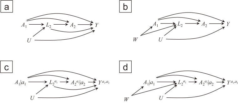
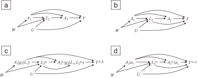
Epidemiologists are increasingly encountering complex longitudinal data, in which exposures and their confounders vary during follow-up. When a prior exposure affects the confounders of the subsequent exposures, estimating the effects of the time-varying exposures requires special statistical techniques, possibly with structural (ie, counterfactual) models for targeted effects, even if all confounders are accurately measured. Among the methods used to estimate such effects, which can be cast as a marginal structural model in a straightforward way, one popular approach is inverse probability weighting. Despite the seemingly intuitive theory and easy-to-implement software, misunderstandings (or "pitfalls") remain. For example, one may mistakenly equate marginal structural models with inverse probability weighting, failing to distinguish a marginal structural model encoding the causal parameters of interest from a nuisance model for exposure probability, and thereby failing to separate the problems of variable selection and model specification for these distinct models. Assuming the causal parameters of interest are identified given the study design and measurements, we provide a step-by-step illustration of generalized computation of standardization (called the g-formula) and inverse probability weighting, as well as the specification of marginal structural models, particularly for time-varying exposures. We use a novel hypothetical example, which allows us access to typically hidden potential outcomes. This illustration provides steppingstones (or "tips") to understand more concretely the estimation of the effects of complex time-varying exposures.
流行病学家越来越多地遇到复杂的纵向数据,其中暴露及其混杂因素在随访期间发生变化。当先前的暴露会影响随后暴露的混杂因素时,估计时变暴露的影响需要特殊的统计技术,可能需要针对目标效果的结构(即反事实)模型,即使所有混杂因素都得到了准确测量。在用于估计此类效果的方法中,这些方法可以直接作为边缘结构模型进行建模,其中一种流行的方法是逆概率加权。尽管理论看似直观,软件易于实现,但仍存在误解(或“陷阱”)。例如,人们可能会错误地将边缘结构模型与逆概率加权等同起来,未能区分编码感兴趣因果参数的边缘结构模型与用于暴露概率的杂项模型,从而未能将这些不同模型的变量选择和模型规范问题分开。假设给定研究设计和测量,感兴趣的因果参数是可识别的,我们提供了广义标准化计算(称为 g 公式)和逆概率加权以及边缘结构模型的规范的分步说明,特别是对于时变暴露。我们使用一个新颖的假设示例,使我们能够访问通常隐藏的潜在结果。这种说明为理解更具体地估计复杂时变暴露的效果提供了垫脚石(或“技巧”)。